Fluid mechanics - ever heard of it?
Our landing page image shows a Kármán vortex streetafter the Hungarian-American physicist von Kármán, 1881-1963. This phenomenon can be observed in fluid mechanics when, for example, a plate is flowed around with a Reynolds numberdimensionless characteristic of the degree of turbulence, after the British physicist Reynolds, 1842-1912 around 100. Here, alternating vortices are created, which lead to pressure fluctuations. These can be so strong that (without appropriate countermeasures) they can cause a bridge to collapse. This is what happened to the Tacoma Bridge in 1940. Your favorite search engine will yield interesting videos.
Fluid mechanicsalso fluid dynamics are part of physics and deal with the laws of all flowing substances, i.e. liquids and gases. The air that surrounds us, the water of the oceans, the blood in our bodies. All of this is unthinkable without fluid mechanics. From these examples it is clear that bodies can be flowed around (e.g. in aerodynamics) or through (e.g. in pipes).
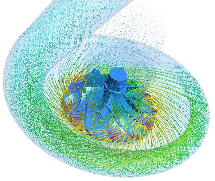
Turbomachinery forms a subfield of fluid mechanics. Within these hydraulic powerPhydr = volumeflow ∙ pressure difference is converted into mechanical powerPmech = torque ∙ angular speed and vice versa. Energy can be added to fluids (e.g. to pump water through a hose), by means of pumps, fans or compressors. The above picture shows the compressor side of a turbocharger, here, as can be assumed, (intake) air is compressed. On the other hand gas, water or wind turbines are used to extract energy from the fluid (e.g. to generate electricity by means of generators within power plants). The quality of the energy conversion is defined as efficiencyη(greek: eta) = Phydr / Pmech (e.g. for pumps). This value is usually given in % and the higher it is, less losses occur in the machine.
You will find fluid mechanics and turbomachinery in all areas of daily life.
This can be seen from some examples below.
Depending on how many aspects you look at, these scopes merge into each other, since machines / devices usually consist of several assemblies / parts:
Energy technology
- Separator / filter unit
- Gas / steam / water turbine
- Heater / heat exchanger
- Wind power plant
Household appliances
- Cooker / cooker bonnet
- Refrigerator / deep fryer
- Hoover / hairdryer
- Washing machine / dryer
Ventilation
- Car / train / air plane
- Computer / electronics
- Underground car park
- Building / Tunnel
Transport / Supply
- Lift / elevator
- Gas / water meter
- Pipeline / valve
- Pump / fan
As you can see, you come into contact with fluid mechanics on a daily basis. And now you know at the latest that „flow“ mechanics does not deal with (flowing) electricity, in any case not directly. In the following, we would like to introduce you to some fundamentals of fluid mechanics, turbomachinery, metrology, computational fluid dynamics, without diving into the world of differentials and integrals. We would like to emphasise that this overview does not claim to be comprehensive.
Fluid mechanics
Technically logical considerations do not always lead to solutions that make sense in terms of fluid mechanics. It can happen that, despite careful consideration, your desired or expected operating point is not achieved in your machine / system. One reason could be swirling flow. The fluid has to cover a longer distance within the pipe, the more swirly the longer. This leads to a higher system resistance / pressure loss. Other potential cause: In a complex system, the loss coefficientsζ (greek: zeta), e.g. for automobiles = resistance coefficient cW ∙ projected area A of the individual components frequently cannot simply be added. Components influence each otherin principle: the smaller the distance, the greater the influence (not only downstream) and thus also the system resistance. With our experience, these challenges - and all others - are quickly and easily coped.
Conservation of mass
Imagine identical vehicles travelling through a tunnel at equal, constant intervals. Identical vehicles have equal masses and also volumes. Equal masses at constant distances can also be interpreted as constant density.
The conservation of mass states that the mass flow(Vehicle) masses per time unit ṁ = Q∙ρmass flow = volume flow∙density is constant over a control volume e.g. said tunnel. In other words, the mass that goes in also comes out again (at the same time). For our example and for the case of incompressibleEven at a depth of 4000 m (i.e. 400 bar pressure), water is only compressed by approx. 2 %. fluids the density is constant. Thus the conservation of mass simplifies to constant flow rate Q = v∙AVolume flow = (average) velocity∙(cross-sectional) area. In our example the cross-sectional area A is equal to the number of lanes.
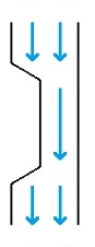
Imagine further that the tunnel has two lanes but in the middle due to a road works only one open. In fluid flows, now something happens that is unbelievable in traffic. Instead of decelerating during threading (and thus causing a traffic jam), the fluid particles accelerate (analogous to the adjacent illustration). Their speed changes inversely proportional to the cross-section. In our case, their speed doubles as the number of lanes is halved.
Bernoulli's theorem
BernoulliSwiss mathematician / physicist, 1700-1782 stated that the total energy of fluid particles along a streamlinee.g. lane in tunnel (filament) is constant. The total pressure is equal to the sum of static, dynamic and geodetic pressure and does not change along the streamline. In pressure notationAlso energy and height notation possible by mathematical conversion this reads: ptot = pstat + pdyn + pgeo = constant .
pgeo = ρ∙g∙Hdensity∙acceleration (on earth)∙height primarily depends on H and is often referred by means of water column (WC2.54 mbar = 1 inch WC = 254 Pa). It is therefore easy to understand that the pressure increasesper 10 m by about 1 bar when diving or that aeroplanes need pressurised cabins because the pressure decreasesper 5,000 m to about half with altitude.
pdyn = ρ / 2∙v² results from the flow velocity and can easily be experienced while blowing on one's own hand or holding it out of the window while driving. In this case the dynamic pressure is converted to a force which pushes your hand back.
pstat is the ambient pressure, on earth − around us − it corresponds to the atmospheric pressure. This is ± 1.013 hPa = 101.300 Pa = 101.300 N / m² ≈ 10,3 tonnes / m² . Therefore we are under a lot of pressure, even without anyone acting on us. However, since the pressure in our bodies is the same, we don't notice it. You can visualize the static pressure by sucking air out of an empty PET bottle. Thus, you lower the pressure inside the bottle and see how it is "magically" compressed by the larger external pressure.
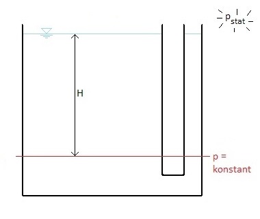
Bernoulli's theorem also vividly shows that the pressure does not depend on the amount of fluid. This is known as the "hydrostatic paradox" (see figure alongside). The pressure along the red line is constant in this open container.
Conservation of momentum
NewtonEnglish polymath, 1643-1727 already stated in his 1st Axiom that a force-freelosses, friction are neglected body moves with constant speed and direction. The speed here can also be zero, which corresponds to a body at rest. In other words: I = m∙vMomentum = mass∙velocity = constant. It can be seen that the momentum changes with the speed. Changes in speed (per unit of time) are caused by acceleration or braking ( = negative acceleration). However, the momentum also changes with the mass. This sounds paradoxical at first, since masses are normally constant. This is due to the fact that we tend to use the LagrangeItalian mathematician, 1736-1813 approach. This is object-related, i.e. one is a co-movingwe are sitting in the moving vehicle (= mass particle) observer. In contrast, the EulerSwiss mathematician, 1707-1783 way of looking at things is location-based, i.e. one is an externalstanding at the road side and watching vehicles passing by observer.
Changes in momentum result in a force effect onto the body. From this follows the 2nd axiom and depending on the point of view: F = m∙aForce = mass∙accelaration or ṁ∙v, respectively.
Turbomachinery
Angular momentum law
The momentum theorem can be adapted for the case of motion on a curved path by means of the location vector r (= radius to the centre of rotation). From this follows the angular momentum conservation: D = r x I = m∙(r x v) . Since only the part of the velocity vector perpendicular to the radius (= vUvU = v∙cos α || uu = r∙ω = r∙2π∙n) contributes to the "leverage", the angular momentum math can be simplified: D = m∙r∙vU . The time derivative of the angular momentum corresponds to the torque: M = ṁ∙r∙vU . After mathematical conversions, you get the power with: P = M∙ωMechanical power = torque∙angular speed = ṁ∙Δ(u∙vU) = Q∙ΔpHydraulic power = volume flow∙pressure difference . Since an ideal machine is considered here, the performances are equal, i.e. the efficiencyη (greek: eta) amounts to 100 %.
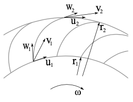
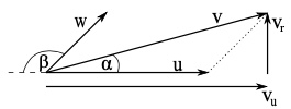
Impellersalso rotors are often designed with the help of so-called speed trianglessee adjacent pictures using the example of forward-curved blades. The absolute = circumferential + relative velocities are vectorially linked via v = u + w. Angle α denotes the absolute and β the relative flow angle (= blade angle). Indices 1, 2 refer to the inlet, outlet of the blade channel. By means of the geometric relationship (Cosine theoremw² = u² + v² − 2∙u∙v∙cos α) and some maths, the turbomachinery equation (SMHGin German: StrömungsMaschinenHauptGleichung) according to Euler can be derived: (u² + v² − w²) / 2 = u∙vU . The left term corresponds to the second and the right term to the first (more common) form.
Integration over the impeller gives: YSpecific supply = P / ṁ = u2∙v2u − u1∙v1u . You recognise the direct connection to the derived angular momentum. If the inflow is swirl-freei.e. v1U = 0, Y becomes maximum. In real machines, the integral quantities (M, ω resp. n, Q, Δp) are measured and the efficiency is determined via the power quotientPmech / Phydr for turbines, Phydr / Pmech for pumps. Which type of turbomachinery (axial, diagonal, radial) should be used for highest efficiency purposes can be determined by means of the CordierGerman Engineer diagram.
Coriolis Force
The CoriolisFrench mathematician and physicist, 1792-1843 force belongs to the apparent or inertial forces and acts on any body that moves within a rotating reference frame. This force can be illustrated by means of the Foucault pendulumaccording to Léon Foucault, French physicist, 1819-1868. Imagine a pendulum (appropriately suspended) swinging close above the ground. Plates are arranged in a circle around the pendulum. It can now be observed that the pendulum does not seem to just swing back and forth. The pendulum is being deflected and it gradually knocks over the plates. In fact, it is the ground (the earth with us as observers on it) that is moving. The Coriolis force can be calculated analogously to Newton's 2nd axiom: FC = m∙aC = -2∙m∙(ω x v) . In this equation, ω corresponds to the angular velocity of the reference frame and v to the velocity of the object moving in it. You can experience the Coriolis force yourself, for example on a turntable (in a playground). Stand facing outwards on the to be rotated turntable. If the disc is spinning constantly, you can stand at ease (assuming it is not spinning so fast that you are experiencing a significant centrifugal force). Now take a step forward and you will be pushed against the direction of rotation, apparently without external influence.
Performance / resistance curves
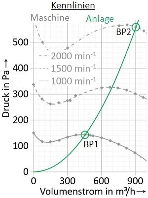
The performance of turbomachinery is often shown by the manufacturer in characteristic diagrams. The example adjacent shows the so-called throttle curves of a centrifugal fan for three operational speeds (gray) and a resistance curve (green). Fans usually move air. You often hear the term blower in colloquial language, but this should not be used in technical language. Correctly it is called fan or compressorfor pressure ratios > 1,3. If not a gas but a liquid is transported, it is called a pump.
The intersection of the throttle and the resistanceusually corresponds to a quadratic function curve yields the actual operating point, here BP1 at 1000 rpm and BP2 at 2000 rpm. Ideally, the machine or generally the machine typee.g. by means of the Cordier diagram should be selected or designed to have the highest possible efficiency in the desired BP. Every Watt that is not consumed does not have to be saved elsewhere and the total cost of ownership (TCO) can potentially be significantly reduced.
If you take a closer look at the example, you will notice that when the rotational speed n doubles, the volume flow Q also doubles and the pressure p quadruples. This behavior can be observed in general and can be described using the affinity laws: Q ∼ n∙D3, p ∼ n2∙D2, P ∼ n3∙D5 . In this example, the required power P thus increases eightfold, but the efficiency (not shown) remains almost unchanged. The affinity laws can also be used to predict the performance of different machine sizes (based on impeller outer diameter D). When the machine size is doubled, Q changes eightfold, p quadruples, and P changes 32-fold.
Computational fluid dynamics
CAD-Model → CFD-Model
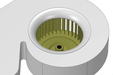
In order to perform flow simulations, it is necessary to derive a fluid volume based on the CAD model. For the case of a fan or a pump (where flow is relevant), all internal surfaces between inlet and outlet are used. As there are no inlet/outlet surfaces in the CAD model, these must be modelled accordingly (e.g. the inlet using a hemisphere). Small gaps (e.g. around the shaft) has to be closed to ensure „tightness“. This creates a closed volume, the actual CFD model. For the fan example, the CFD model must be subdividedinto so-called regions or domains, because this model consists of rotating and stationary areas. For parameter studies, very large models or to exploit symmetries, the CFD model should also be segmented (sensibly). The bottom line is that this reduces the time required for meshing. Meshing is also called grid generation. Appropriate care at this point can avoid unnecessary headaches in the following step.
Meshing (grid generation)
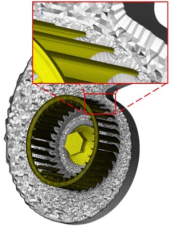
The mesh is created by dividing the fluid volume into many small control volumes (up to several millions). For each of these control volumes, the mass, momentum and (if required) energy conservation equations are solved during the calculation iteratively. Nowadays, meshes are generated using tetra-, prism-, hexa-, or polyhedron cells. Although (semi-)automatic meshers have become more powerful in recent years, their results must always be checked critically. As before, only the specifications / settings of the experienced user lead to high-quality meshes. The mesh quality can be checked by means of suitable control variables, like Aspect Ratio, Volume Change or (smallest orthogonal) angles within the cells.
In order to be able to calculate (and not just model) near-wall flows, a corresponding near-wall mesh resolution is necessary. The quality of this so-called boundary layer resolution is described by means of the dimensionless wall distance y+. The order of magnitude of the y+ value depends on the used turbulence modelling. For the in industry mostly used SSTShear Stress Transport or realizable-k-ε turbulence models, the value should be below two. Logically, for different operating points (flow velocities), the y+ value is also different (despite identical mesh). The adjacent figure shows a section through a typical mesh (tetrahedrons incl. prism boundary layer, impeller diameter 90 mm).
For structural simulations, „only“ the actual CAD model is meshed. This is one reason why the effort is significantly lower than for flow simulations. There is also no need for near-wall resolution or turbulence modelling here.
Steady-state and transient calculations (simulations)
For industrial applications, stationarytime independent calculations should always be used (if possible). The background is that transienttime-dependent calculations (on average) take 20 timesURANS vs. RANS longer without generating more significant information. In the case of a pump or fan calculation, it is usually not relevant to know how the pressure build-up changes with each millisecond (see video on the left). If this machine is investigated experimentally, you will usually end up with only one (average) value for pressure build-up, driving power and efficiency.
For stationary calculated rotating machines, the blade forces are modelled via the Coriolis forces. This is necessary because the impeller does not rotate here. If the number of blades is high enoughhow high depends on the case, this is acceptable. However, the situation is different if the number of blades is too low. In the extreme case of a sewage pump with only one blade channelthis lowers the risk of blocking, the calculation results are very dependent on the impeller position, because of the interaction with the scroll. In such cases, I guess you have to perform transient calculations. Or try the following „trick“: Calculate several impeller positions in steady-state and then average these results. This often gives you the information you need and you still save time compared to transient calculations.
Transient calculations are therefore more likely to be found in the field of research, for example when the influence of time-limited phenomena is to be investigated.
Here, significantly more complex turbulence modelling (e.g. LESLarge Eddy Simulation, DESDetached Eddy Simulation, DNSDirect Numerical Simulation) is used, which again significantly increase the required time.
Instationary effectsInstabilities,
e.g. high pressure fluctuations in stationary calculations can already be detected during the calculation on the basis of the residuals and suitable monitors.
If (undesirable) transient effects occur in your product, you should determine the cause and counteract, e.g. with a geometry adjustment.
„Special“ simulations
In „usual“ calculations, the entire CFD model is filled with only one fluid (e.g. air or water). VOFVolume of Fluids calculations allow the use of multiple fluids within one CFD model. By this, the inflow behaviour of water into an air filled tank can be calculated (see video on the right). VOF can also be used to study the behaviour of solids within fluids. One application could be the calculation of ship movement at sea (two fluids, one solid). It goes without saying, that VOF calculations are always transient.
FSIFluid Structure Interaction calculations couple flow and structure simulations, i.e. the interaction between fluids and solids. This means that, e.g. forces resulting from the flow are transferred to the FEMFinite Element Methode model. Using these forces, the stress distribution within and the deformation of the component is calculated. The calculated deformation (geometry change) can be fed back into the CFD model and the flow will be recalculated based on this.